Pivot tables are an incredibly useful tool for data analysis, and they can be used in a variety of different ways. If you’re new to pivot tables, or if you’re looking for a refresher on how to create one, this blog post is for you. We’ll walk through a few different examples of how to create a basic pivot table so that you can get a better idea of how they work and how they can be used. By the end of this post, you should have a good understanding of what pivot tables are and how to create one yourself.
A pivot table is a powerful tool that allows you to summarize data in a way that you can easily understand and interpret. It is essentially a way to take data from a large table and rearrange it so that it is easier to see the relationships between different pieces of information.
For example, let's say you have a table with data on sales of different products in different regions. With a pivot table, you could easily see which products are selling well in which regions. You could also see how sales have changed over time for each product.
Pivot tables are extremely flexible, and there are many different ways that you can use them. This article will show you how to create a basic pivot table in Excel.
When you create a pivot table, you are essentially taking a large data set and summarizing it in a way that is easy to understand and interpret. A pivot table takes data from one or more columns in a data set and aggregates it across the columns to produce a summary.
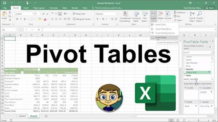
To create a pivot table, you first need to select the data that you want to summarize. You can do this by clicking on the cells in the data set or by selecting a range of cells. Once you have selected the data, click on the Insert tab and then click on Pivot Table.
In the Create PivotTable dialogue box, choose where you want to place the pivot table and then click OK.
Next, you need to choose which fields you want to include in the pivot table. To do this, drag and drop the fields from the field list into either the Row Labels or Column Labels area. You can also drag fields into the Values area if you want to include them in the pivoted data.
Once you have added all of the fields that you want to include, click on OK. Your pivot table will be created!
A pivot table is a powerful tool that allows you to summarize large amounts of data. Pivot tables are used to create summary reports from raw data. The data is arranged in a tabular format and the user can select which columns to include in the report and how to group the data.
Pivot tables are commonly used to analyze financial data, but they can be used on any type of data set. For example, you could use a pivot table to analyze survey results or customer data.
Pivot tables are a flexible way to summarize data and can be customized to show only the information that you want to see. For instance, you can choose to show only the total number of responses for each question or you could choose to show the percentage of people who answered each question.
Pivot tables are a helpful tool for understanding complex data sets. They can be used to identify trends and patterns that would be difficult to spot using other methods.
A pivot table is a powerful way to summarize data in Excel. It can be used to calculate count, sum, average, and other statistics for data in your worksheet. You can also use it to filter and sort data and create charts based on your pivot table data.
To create a pivot table in Excel:
1. Select the data you want to use in your pivot table. This can be any range of cells in your worksheet or even an entire worksheet.
2. Click the Insert tab on the ribbon, and then click Pivot Table in the Tables group.
3. In the Create PivotTable dialogue box, choose where you want to add your new pivot table. The default location is a new worksheet, but you can also choose to place it in an existing worksheet.
4. Click OK to create your pivot table.
5. In the PivotTable Field List pane that appears on the right side of your screen, drag-and-drop the fields you want to use in your pivot table into the appropriate areas:
* Drag fields into the Row Labels area to create rows in your pivot table.
* Drag fields into the Column Labels area to create columns in your pivot table
* Drag fields into the Values area to calculate statistics for those fields

So, you've got a killer business idea. But when you sit down to name it, you hit a wall. Every...

Whether you're feeling curious, looking for a friendly conversation, or hoping to meet someone...

For most people, their smartphones and other end-user devices are their portals into the digita...

The sun is your best friend when it comes to powering your home. After all, it provides free, r...

In the current business scenario, a mobile app has become a need for every business. It helps y...

As a small business owner, you know that inventory management is crucial to your success. After...